CS134 Project Milestone Report
A Machine
Learning System for Stock Market Forecasting
My email: Jianfeng.Huo@dartmouth.edu
Motivation:
Recently,
a large amount of amazing work has been done in the area of analyzing and
predicting stock prices and index changes using Machine Learning Algorithms.
Intelligent Trading Systems has been used for most of the stock traders to help
them in predicting prices based on various situations and conditions, thereby
helping them in making instantaneous investment decisions. Stock market
prediction is regarded as one of the most challenging task in financial
time-series forecasting. This is primarily because the underlying nature of the
uncertain financial domain and in part because of the mix of known parameters
(Previous Day’s Closing Price, P/E Ratio etc.) and unknown factors (Election
Results, Rumors etc.).
In my project, I will implement a machine learning
system which is proposed by Lijuan Cao and Francis
E.H. Tay [1] based on Support Vector Machines (SVMs)
for stock market prediction. SVMs were originally developed by Vapnik for
pattern recognition problems. In this case we try to find an optimal hyperplane
that separates two classes. In order to find an optimal hyper plane, we need to
minimize the norm of the vector w, which defines the separating hyper
plane. This is equivalent to maximizing the margin between two classes.
Recently with the introduction of ε-insensitive loss function, SVMs has been
extended to solve non-linear repression problems. In the case of regression,
the goal is to construct a hyperplane that lies "close" to as many of
the data points as possible. Therefore, the objective is to choose a hyperplane
with small norm while simultaneously minimizing the sum of the distances from
the data points to the hyperplane. Both in classification and regression, we
obtain a quadratic programming problem where the number of variables is equal to
the number of observations [4].
Method:
Regression
approximation emphasizes the problem of estimating a function based on a given
set of data ![]() (xi is the input vector and di is the desired
value), which is produced from the unknown function. SVMs approximate the
function in the following form:
(xi is the input vector and di is the desired
value), which is produced from the unknown function. SVMs approximate the
function in the following form:
Where
![]() are the features of inputs and
are the features of inputs and ![]() , b are coefficients. Thus they are estimated by minimizing the
regularized risk function (2):
, b are coefficients. Thus they are estimated by minimizing the
regularized risk function (2):
In
equation (2), the first term ![]() is the ε-insensitive loss
function. It is a self-explanatory function that indicates the fact that it
does not penalize errors below ε. The second term
is the ε-insensitive loss
function. It is a self-explanatory function that indicates the fact that it
does not penalize errors below ε. The second term ![]() is used as a measure of
function smoothness. C is a prescribed constant representing determining the
trade-off between the training error and model smoothness. Introduce slack
variables ζ, ζ* to the above equations we have the following
constrained function:
is used as a measure of
function smoothness. C is a prescribed constant representing determining the
trade-off between the training error and model smoothness. Introduce slack
variables ζ, ζ* to the above equations we have the following
constrained function:
Minimize:
Subject to:
![]()
![]()
![]()
Thus, Eq. (1) becomes the following explicit form:
Lagrange Multipliers.
In
function (5), ![]() are the Lagrange multipliers
introduced. They satisfy the
are the Lagrange multipliers
introduced. They satisfy the ![]() equality
equality![]() , and they can be obtained by maximizing the dual form of function
(4), which has the following form:
, and they can be obtained by maximizing the dual form of function
(4), which has the following form:
With the following constraints:
![]()
![]()
This
is a quadratic programming problem and only a number of coefficients ![]() will be assumed to be nonzero
and the data points associated with them can be referred to as support vectors.
will be assumed to be nonzero
and the data points associated with them can be referred to as support vectors.
Experiment:
The SSEC Index in Shanghai Mercantile is selected for the
experiment. We choose Every Wednesday’s Close price adjusted for dividends and
splits from Apr. 19th, 1999 to Oct. 15th,
2001 as the input data for the experiment. The main reason for choosing this
period is that it contains an obvious collapse during this period which is
shown in figure 1. We use ε-SVM to train the first 80 data and then predict the
rest of the data. The error of the training and predicting procedure is
measured by Root-Means-Square-Error (![]() )
)
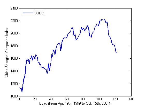
Figure
1- Index of SSEC (Apr. 19th, 1999-Oct. 15th,
2001)
Before predicting we did a simple preprocessing with the original
data. As unusually done in the economic analysis, we did a logarithmic
transformation to the data and then scale it into the range of [0, 1]. We
choose Gaussian Radial function as the kernel function in the experiment. For
each train set, we use the previous six days’ data to predict the seventh day’s
price. There are 74 sets of training data (i.e. 80 days’ market indices) that
is to say we will discover and memorize the sequence’s statistical law through
the previous 80 days’ data and predict the rest days’ indices in the period.
The result is shown in figure 2. The blue line represents the actual index of
the market and the red stars represent the output from the SVM. The training
error is 0.0061 and the testing error is 0.0078.
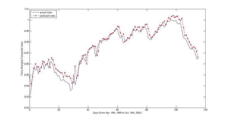
Figure 2-experiment result
To do:
l • Add more technical indicators as the input features
l • Have a study of the sensitivity of SVMs to parameters
l • Apply the system to more stock markets, e.g. DJI
Timeline:
l Read papers about using SVM for stock market prediction
l Before milestone implement the hybrid machine learning system in Matlab.
l Before final debug the algorithm, test data and improve accuracy of the system.
l Analyze experiment results and write the final report.
Reference
[1] L. J. Cao and F. E. H. Tay, "Financial
forecasting using support vector machines", Neural Comput.
Applicat., vol. 10, no. 2, pp. 184-192, 2001.
[2] Vatsal H. Shah, “Machine Learning Techniques for Stock Prediction”, http://www.vatsals.com/Essays/MachineLearningTechniquesforStockPrediction.pdf
[3] R. Choudhry and K. Garg, "A hybrid machine learning system for stock
market forecasting," Proceedings of World Academy of Science, Engineering
and Technology, vol.29, pp. 315-318, 2008.
[4]T. B. Trafalis and H. Ince. Support
vector machine for regression and applications to financial forecasting.
IJCNN2000, 348-353
[5] http://in.finance.yahoo.com/